What is Hamilton-Jacobi (HJ) Reachability Analysis?
The Brief Explanation
An animation of how we produce a reachable set. First the goal (or unsafe set) is defined, shown here as the blue circle. We then create a level set function that is a signed distance function: negative inside the set and positive outside. We propagate this function using HJ reachability for the desired time horizon. Finally, we take the zero slice of this function to produce the reachable set
HJ reachability analysis is all about optimal control and guarantees for reaching goals and staying safe. When given:
1) a dynamic system with input bounds (e.g. robot, car, biological system),
2) goal and/or failure region(s), and
3) bounds on uncertainties or adversaries that impact the system,
this method produces a scalar value function.
Given the current state of the system (e.g., the position and velocity information of the robot), the value function outputs a scalar number that corresponds to whether the problem (reaching the goals and/or avoiding the obstacles) is achievable. Moreover, the gradient of the value function informs the direction that the system must go in order to behave optimally, even in the face of worst-case behavior from adversaries or uncertainties in the system/environment.
The Thorough Explanation
Please see our tutorial paper for a more thorough introduction.
Why Study HJ Reachability?
Once a value function is computed, it can very quickly be used to assess:
1) From what initial conditions is your goal reachable / obstacle avoidable?
2) Given the current state of the system, what input should be applied to optimally reach the goal and/or avoid the obstacles?
This is extremely useful in safety-critical scenarios. When flying a plane or administering anesthetics, accidental mistakes from less rigorous planning methods can result in disaster. Reachability is able to provide guarantees on what is safe, as well as how to implement controls to accomplish your goal. What’s more, HJ Reachability can handle nonlinear dynamics and worst-case external disturbances.
The main challenge of HJ reachability lies in its computational cost. Due to the nature of dynamic programming, the computational complexity of solving a reachability problem rises exponentially with the number of dimensions in the system. We have several works that tackle this problem from a control-theoretic perspective using tools like decomposition or reduced order models. We also have approaches that incorporate learning-based approaches that provide scalable approximations at high dimensions. These learning-based approximations can then be used by our more classical approaches to provide safety and goal-satisfaction guarantees.
Theory papers from our Group
These papers cover how HJ reachability relates to other approaches for safety analysis and control, and how it can be applied beyond its original problem formulation.
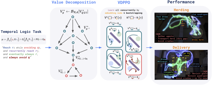
Generalizing HJ Reachability to Temporal Logic Specifications
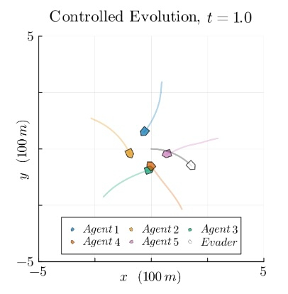
In these papers, we show how HJ reachability can be used for general task logic. For example, in the hardware experiment below, the two quadcopters must “deliver” packages to random goals while avoiding obstacles and a no-fly zone (the square in the center). They must also regularly “charge” by flying over the quadruped. This kind of long-horizon complex task can be specified using temporal logic. However, solving these temporal logic problems for control is challenging.
We have some nice results showing how we can decompose such specifications into small sub-problems that are easier to learn/compute. Importantly, when we recompose the solved value functions, the resulting value function satisfies the original task specification.
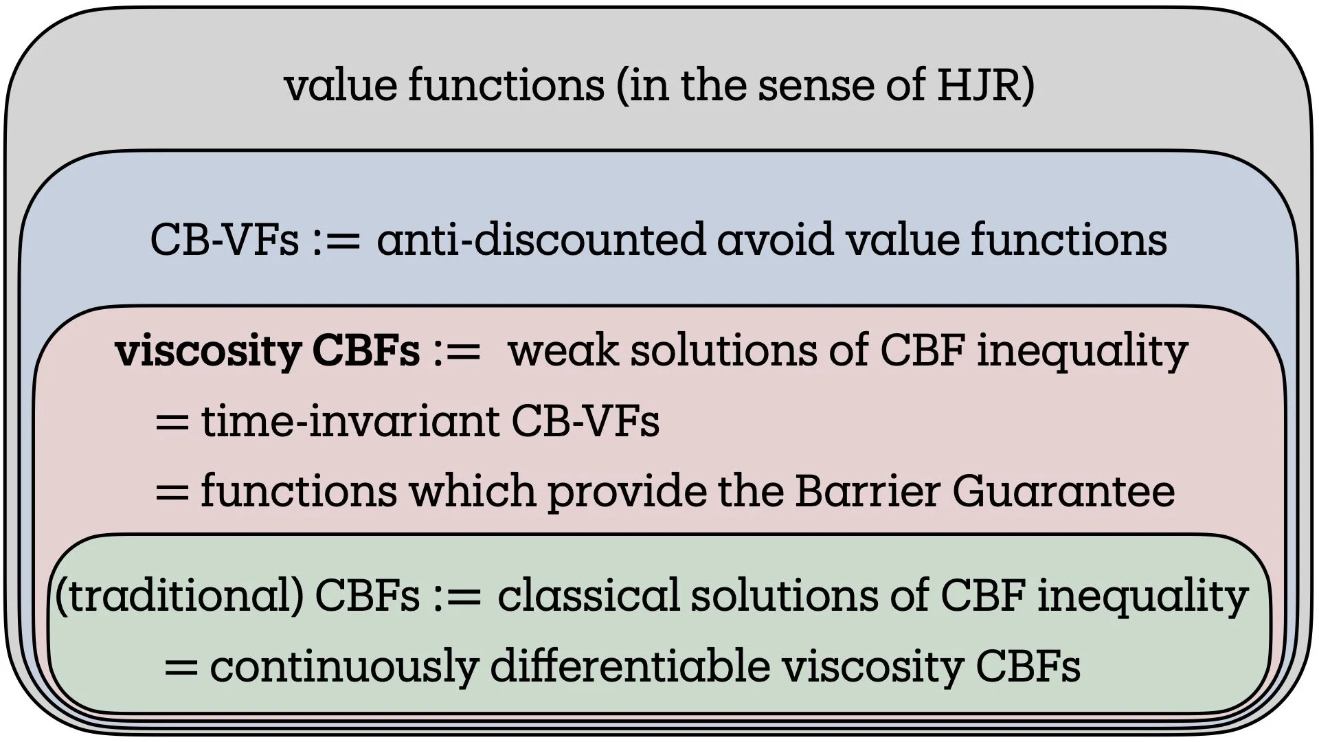
On the Relationship between Hamilton-Jacobi Reachability and Control Barrier Functions
A specific use case of HJR is to generate a value function that can act as a safety filter. Safety filters are used to minimally modify a nominal control input to maintain safety. These have gotten very popular, as companies often want to add a safety “wrapper” to a performance layer that doesn’t guarantee safety (e.g. foundation models, video-language-action models, etc.). More on this on the safety filter page.
Another common safety filter is called a control barrier function (CBFs). We took a deep dive into understanding the relationship between CBFs and HJR, and how the two approaches can be used together to strengthen the theoretical underpinnings and practical tools for each method.
HJ Reachability for Stabilization Problems
Traditional HJR solves for the minimum time to reach a goal. This is useful in many applications, but not all. For example, reaching a parking space in the minimum time would involve accelerating straight through the parking space. In many cases, we want to ensure that the system not only reaches a goal, but stabilizes there. The following works explore how to formulate this using HJR.
Solving Reach- and Stabilize-Avoid Problems Using Discounted Reachability [TAC 2026]
Constructing Control Lyapunov-Value Functions Using Hamilton-Jacobi Reachability Analysis [LCSS 2023]
Papers on Tools for Solving Reachability
Learning-based approaches for scalability
To extend the scalability of HJR, one of the most promising approaches is via learning-based methods. The challenge is how to encourage goal-reaching and obstacle-avoiding behavior when learning over high-dimensional state spaces. We have several approaches to this.
For reinforcement learning, we can a) propose special safety Bellman equations that can decompose rigorously into smaller problems with richer reward functions that are easier to learn, b) incorporate adversarial players during learning for robustness, and c) encourage the system to return efficiently to safety when it is in danger.
For supervised learning, we have work showing that we can a) guide the training using supervision from linear methods or model-predictive control, and b) locally patch small invalid regions of the value function using HJR, recovering guarantees.
Reinforcement Learning
Supervised Learning
Transformation to linear spaces (e.g. Koopman)
This paper employs a tool from the applied math community (Hopf reachability) to perform very fast reachability analysis. The catch is that this tool requires the system to be linear time varying. By linearizing a nonlinear system (by lifting it to a higher dimension), we can bound the resulting linearization error and treat this error as an adversarial disturbance in the reachability computation. This results in guaranteed conservative results on the true nonlinear system with the speedup available using the linear approach.
Decomposition-based Approaches
By decomposing the dynamic system either in space or time, we can solve smaller sub-problems.
Decomposition in time
Decomposition in space
Reduced order modeling
We have shown that by solving a game between a high-fidelity model of a system and its low-dimensional reduced-order model, we can use the precomputed solution to augment any low-dimensional planner with a tracking error bound and tracking controller on the high-fidelity system. This allows us to plan in low dimensions with safety guarantees on the high-dimensional system. For more details, see the FaSTrack page.
Available Toolboxes
hj_reachability (Python) — this is the Python implementation of the above toolboxes, led by Edward Schmerling at Stanford. It is much more efficient than the MATLAB version and has an active group maintaining and updating it. It currently lacks some of the niche functionality of the helperOC toolbox below, but it is very good for most reachability applications and is adding new functionality rapidly.
helperOC (MATLAB) — Our public code for computing reachable sets can be cloned or downloaded at https://github.com/HJReachability/helperOC (note: this is essentially a user-friendly wrapper with extra functionality for Prof. Ian Mitchel’s level set toolbox). This MATLAB repository contains a lot of visualization functionality. The downside is that it is not as efficient as the other toolboxes.
DeepReach (Python) — Toolbox from Prof. Somil Bansal at the University of Southern California for approximating high-dimensional value functions using sinusoidal neural networks. Paper here.
BEACLS (C++) — BEACLS stands for Berkeley Efficient API in C++ for Level Set methods. It is essentially a reimplementation of the MATLAB toolboxes in C++ with tweaks to improve efficiency and compatibility with GPUs. It is quite a bit faster than the MATLAB implementation, but sacrifices readability for performance.
optimized_dp (Python/C++) — This toolbox was built by Prof. Mo Chen at Simon Fraser University, with the goal of having an easy python-based user interface to set up a reachability problem, and then conversion to fast C++ code via HeteroCL.
Flow* — Developed by Prof. Sriram Sankaranarayanan at CU Boulder. Good for computing safe sets for large numbers of states, and computing sets that do not have control/disturbance inputs (i.e. policy is already determined and plugged into dynamics). Uses scalability tools that lead to over-approximation of reachable sets.