What are Safety Filters?
The Brief Explanation
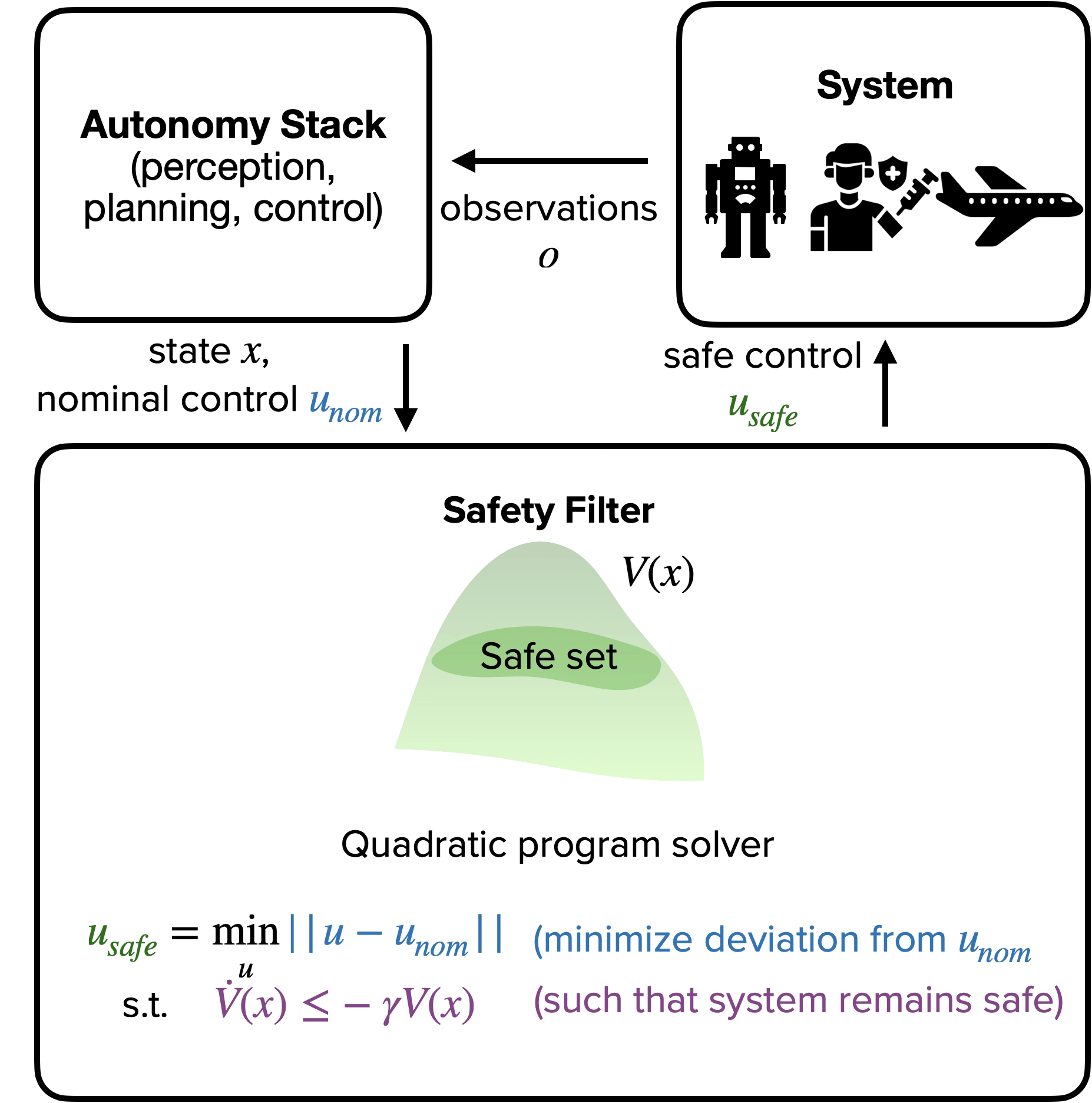
As a community, we are relying more and more on planning and control stacks that rely on black-box and data-driven approaches. While sometimes more performant, these methods generally 1) are not explainable (i.e. it’s hard to follow their logic), and 2) cannot guarantee that they will generate safe control actions. Because of this, there has become more and more demand for a standalone “safety module” that can wrap around this autonomy stack and ensure that the resulting action to the system is safe. This is the basic idea for safety filters.
A safety filter takes in the current state of the system and the desired control action from the planning and control stack. The filter, if designed correctly, will minimally modify this desired action to ensure safety. For a large class of systems, this optimization is a “quadratic program,” and can be solved very quickly during runtime.
The filter depends on a key function, often called a Control Barrier Function, Safety Value Function, or sometimes we directly call it the Safety Filter. This function is designed based on the system dynamics and the safety constraints. It has two very important features:
The function takes in the current state of the system, and outputs the current safety level. Positive is safe, negative is unsafe (i.e. may lead to failure).
The gradient of the function informs the set of control actions that are allowed, i.e. that preserve safety.
These two pieces of information are used in the filter to assess current safety levels and to modify the performance control action to stay within the set of safety-preserving actions. (aside: if you are familiar with control Lyapunov functions, these are intimately related).
There are a few challenges with safety filters, but by far the biggest challenge is how to find a valid safety filter. This is especially hard when: a) the system is high-dimensional, b) the system has complicated dynamics (e.g. nonlinear, high-order), c) the system has bounded inputs and/or disturbances, and d) the safety constraints are complicated. This motivates the use of constructive methods like Hamilton Jacobi Reachability to compute these functions. We have work on connecting the theory of different safety filter approaches so that we can use all our work on scaling Hamilton-
The Thorough Explanation
Here is a nice survey on safety filters from 2024 from Professor Jaime Fisac and his group.
Here is a comparison of several approaches for data-driven safety filters from 2023, written by several experts in the field.
For deeper theory connections, I am quite partial to my student Dylan Hirsch’s recent paper from 2026.
Theory papers from our Group
On the Relationship Between Different Kinds of Safety Filters
There are a few commonly used safety filters in the literature:
Artificial Potential Fields (APFs), popularized in the 80’s, are the simplest and apply to simple kinematic systems. They essentially pretend that your system is a magnet that feels a repulsive force from other obstacles and an attractive force towards goals.
Control Barrier Functions (CBFs), are generalized artificial potential fields that handle more realistic nonlinear dynamics. Fun fact: they are essentially “upside down” control Lyapunov functions (CLF): outside of the safe set, the CBF acts exactly like a CLF. Inside the safe set, the same exponential decay requirement from the CLF condition now acts to prevent the system from leaving the safe set.
Hamilton-Jacobi Reachability can produce Safe Value Functions that have many similar properties to CBFs.
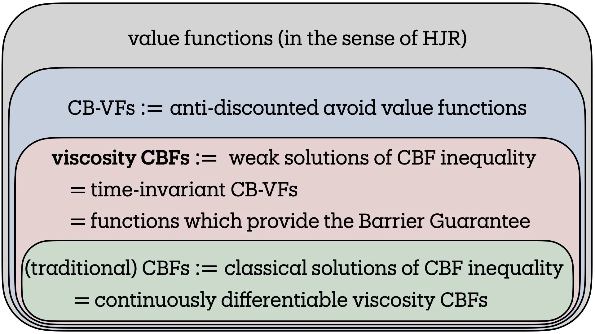
We have a line of work showing that Hamilton-Jacobi-Reachability can construct functions that are a generalization of standard control barrier functions. We term these “Viscosity Control Barrier Functions.” Related papers:
Robust Control Barrier–Value Functions for Safety-Critical Control [CDC 2021]
A Forward Reachability Perspective on Robust Control Invariance and Discount Factors in Reachability Analysis [under review]
Extending Safety Filter Theory: Reach-Avoid, Time Varying, Compositional
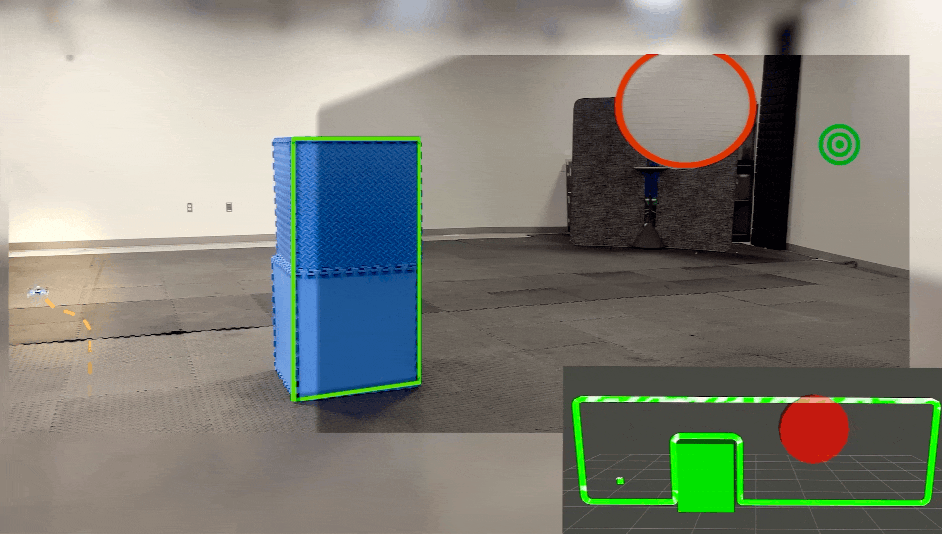
We have extended the notion of a safety filter beyond a static function guiding the system away from fixed safety constraints. We now have filters that: a) guide the system not just away from obstacles, but towards goals, b) are time-varying, enforcing stricter constraints over time in order to, e.g., force a robot to return to its charging port at the end of the time horizon, c) adapt with changing environmental disturbances, and d) combine to allow for contingency planning (i.e., at least one safe backup set should be reachable).
Solving Reach- and Stabilize-Avoid Problems Using Discounted Reachability [TAC 2026]
Back to Base: Towards Hands-Off Learning via Safe Resets with Reach-Avoid Safety Filters [L4DC 2025]
Constructing Control Lyapunov-Value Functions Using Hamilton-Jacobi Reachability Analysis [LCSS 2022]
From Space to Time: Enabling Adaptive Safety with Learned Value Functions via Disturbance Recasting [CoRL 2025]
Steering with Contingencies: Combinatorial Stabilization and Reach-Avoid Filters [under review]
Papers on Computing Safety Filters from our Group
Warm-Starting for Refining Safety Filters
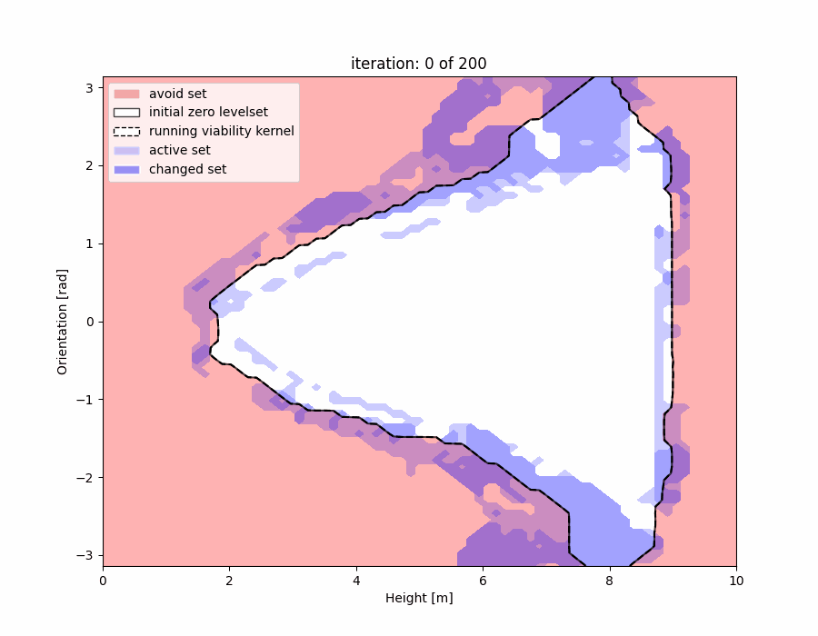
A challenge with safety filters is how to modify them when either a) the initial function is incorrect, or b) the safety constraints change during deployment.
The first case happens often: common approaches to generate safety filters include guess-and-check with simplified dynamics or assumptions on inputs, or data-driven approaches. Both often result in close but invalid safety filters. The second case also occurs frequently, particularly when information about the environment the system operates in changes during deployment.
We show that, rather than computing a safety filter from scratch, we can “warm-start” our computation with the “close but invalid” safety filter in hand. We have examples showing how we update the safety filter on the fly during deployment, and also how we “patch” data-driven safety filters locally in the regions where they are invalid:
Learning Better Safety Filters Offline
Warm-starting works well when we have a “close” initial safety filter to refine. This motivates making data-driven safety filters as accurate as possible. We have several approaches for generating safety filters using both supervised learning with physics-informed neural networks, as well as safe reinforcement learning. See more details on the Hamilton-Jacobi Reachability page.
Reachability Barrier Networks: Learning Hamilton-Jacobi Solutions for Smooth and Flexible Control Barrier Functions [under review]
Back to Base: Towards Hands-Off Learning via Safe Resets with Reach-Avoid Safety Filters [L4DC 2025]
From Space to Time: Enabling Adaptive Safety with Learned Value Functions via Disturbance Recasting [CoRL 2025]
Learning Safety Filters Online Due to Uncertainty in System Dynamics, Measurements, etc.
A system may need to adapt its safety filter during deployment because of noise in perception or uncertainty in the system’s dynamics. In these cases, online learning techniques like Gaussian Processes are attractive because they can provide probabilistic bounds on safety. However, these methods are not scalable and are cumbersome to use online. We have several papers on how to improve scalability using, for example, event-triggered learning and object-centric representations.
Object-Centric Representations for Interactive Online Learning with Non-Parametric Methods [CASE 2023]
Sensor-Based Distributionally Robust Control for Safe Robot Navigation in Dynamic Environments [IJRR 2026]
Learning High-Order CBFs using Gaussian processes for systems in Brunovský canonical form [CDC 2025]
Safe Event-triggered Gaussian Process Learning for Barrier-Constrained Control [TAC 2026]
Safe Event-Triggered Learning for Sampled-Data Systems [ACC 2026]
Expanding Safe Sets with Learning-Based Barrier Functions and Reachability [under review]
Model-Free Safety Filters for Hard-to-model Interaction Effects
Many of the approaches above assume access to a model of the system dynamics. This is often reasonable, but there are many cases where models are challenging or impossible to construct. For example, social interaction effects between pedestrians in a crowd, or contact dynamics when navigating through a cluttered workspace. In these cases, we have worked on approaches for implicitly capturing these unmodeled effects into the structure of the safety filter.
Sequential Neural Barriers for Scalable Dynamic Obstacle Avoidance [IROS 2023, RoboCup Best Paper Award]
Learning to Nudge: A Scalable Barrier Function Framework for Safe Robot Interaction in Dense Clutter [under review]
Papers on Applications of Safety Filters
In addition to the standard applications we have used in the group (walking robots, flying robots, driving cars/robots), we have also used our safety filters for applications in other groups.
Haptic Virtual Fixtures for Telemanipulation using Control Barrier Functions [Transactions on Haptics]